Elevate LLM Embeddings: 7 Advanced Feature Engineering Techniques

Mastering model.encode(text) is just the beginning. This article unveils seven potent, practical strategies to elevate raw Large Language Model (LLM) embeddings into exceptional, task-specific features, significantly boosting downstream model performance. We will leverage robust libraries such as scikit-learn and sentence-transformers to translate advanced concepts into actionable code.

Modern LLMs generate sophisticated vector representations (embeddings) capturing profound semantic nuances. While these embeddings offer immediate performance gains, a critical gap often exists between general semantic knowledge and the precise signals required for your unique prediction objectives. Advanced feature engineering bridges this chasm. By ingeniously processing, comparing, and decomposing these fundamental embeddings, we extract hyper-relevant information, mitigate noise, and equip your downstream models with truly impactful features. Embrace these seven transformative techniques to close the embedding gap.

The Embedding Advantage: Unlocking Task-Specific Power

You've successfully encoded text into numerical representations. Now, how do you harness that power for specific tasks? This guide reveals seven advanced, practical techniques to transform generic LLM embeddings into high-signal, task-specific features that dramatically enhance downstream model performance. We'll cover essential topics including:

• Constructing interpretable similarity features using concept anchors.
• Purifying embeddings through reduction, normalization, and whitening to eliminate noise.
• Generating sophisticated interaction, clustering, and synthesized features.

Let’s dive in.

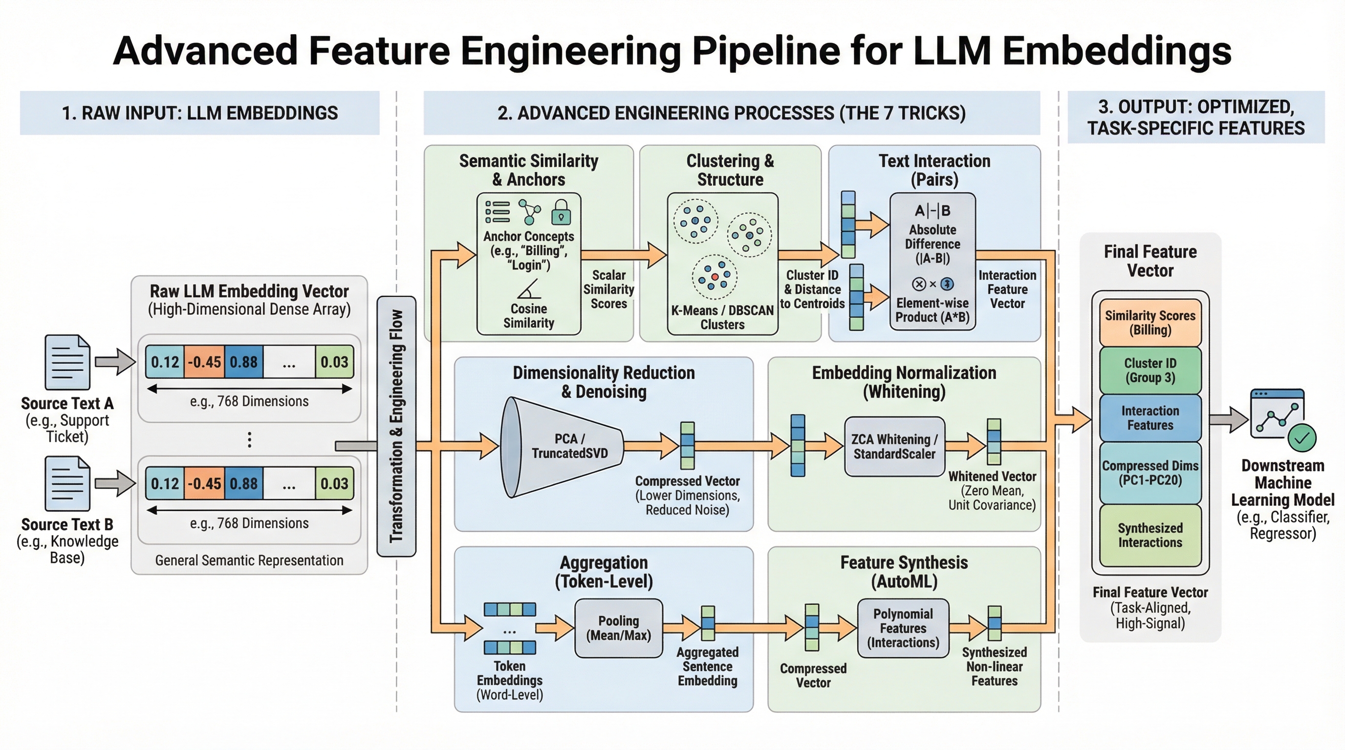
7 Advanced Feature Engineering Tricks Using LLM Embeddings
Image by Editor

1. Semantic Similarity as a Feature

Elevate single embedding vectors into interpretable, scalar features by computing their similarity against critical concept embeddings relevant to your problem. For instance, an urgency classification model for support tickets must discern if a ticket pertains to "billing," "login failures," or "feature requests." Raw embeddings contain this semantic information, but a standard model cannot directly access it.

The solution involves establishing concept-anchor embeddings for pivotal terms or phrases. For each piece of text, calculate its cosine similarity to each anchor embedding. This quantifies relevance, furnishing your model with focused, human-interpretable signals regarding content themes.

Begin by installing the necessary libraries. Execute the following command in your terminal:

pip install sentence_transformers sklearn numpy

from sentence_transformers import SentenceTransformer
from sklearn.metrics.pairwise import cosine_similarity
import numpy as np


model = SentenceTransformer('all-MiniLM-L6-v2')
anchors = ["billing issue", "login problem", "feature request"]
anchor_embeddings = model.encode(anchors)


new_ticket = ["I can't access my account, it says password invalid."]
ticket_embedding = model.encode(new_ticket)


similarity_features = cosine_similarity(ticket_embedding, anchor_embeddings)
print(similarity_features)  

Careful anchor selection is crucial. Derive anchors from domain expertise or employ clustering techniques (see "Cluster Labels & Distances as Features").

2. Dimensionality Reduction and Denoising

High-dimensional LLM embeddings (often 384 or 768 dimensions) can introduce noise and computational overhead. Reducing dimensionality not only purges extraneous noise but also prunes computational costs and can surface more precise patterns.

The "curse of dimensionality" impairs models like Random Forests when numerous dimensions lack informative value. Employ scikit-learn’s decomposition techniques to project embeddings into a more manageable, lower-dimensional space.

First, define your text dataset:

text_dataset = [
    "I was charged twice for my subscription",
    "Cannot reset my password",
    "Would love to see dark mode added",
    "My invoice shows the wrong amount",
    "Login keeps failing with error 401",
    "Please add export to PDF feature",
]

from sklearn.decomposition import PCA, TruncatedSVD
from sklearn.manifold import TSNE  


embeddings = np.array([model.encode(text) for text in text_dataset])



n_components = min(50, len(text_dataset))
pca = PCA(n_components=n_components)
reduced_pca = pca.fit_transform(embeddings)


svd = TruncatedSVD(n_components=n_components)
reduced_svd = svd.fit_transform(embeddings)

print(f"Original shape: {embeddings.shape}")
print(f"Reduced shape: {reduced_pca.shape}")
print(f"PCA retains {sum(pca.explained_variance_ratio_):.2%} of variance.")

The PCA technique excels by identifying axes of maximal variance, effectively encapsulating the most significant semantic information within fewer, uncorrelated dimensions. While dimensionality reduction is inherently lossy, rigorous testing is essential to confirm whether reduced features maintain or enhance model performance. PCA operates linearly; for nonlinear relationships, consider UMAP (though be mindful of its hyperparameter sensitivity).

Original shape: (6, 384)
Reduced shape: (6, 6)
PCA retains 100.00% of variance

3. Cluster Labels and Distances as Features

Leverage unsupervised clustering on your collection of embeddings to uncover inherent thematic groups. Utilize cluster assignments and distances to cluster centroids as potent new categorical and continuous features. This method addresses the limitation where data may contain emergent categories not covered by predefined anchors, providing structural knowledge about natural data groupings, which is invaluable for classification or anomaly detection.

from sklearn.cluster import KMeans, DBSCAN
from sklearn.preprocessing import LabelEncoder



n_clusters = min(10, len(text_dataset))
kmeans = KMeans(n_clusters=n_clusters, random_state=42)
cluster_labels = kmeans.fit_predict(embeddings)


encoder = LabelEncoder()
cluster_id_feature = encoder.fit_transform(cluster_labels)


distances_to_centroids = kmeans.transform(embeddings)  




enhanced_features = np.hstack([embeddings, distances_to_centroids])

The number of clusters (k) is a critical choice, guided by methods like the elbow method or domain expertise. DBSCAN offers a density-based clustering alternative that bypasses the need to pre-specify k.

4. Text Difference Embeddings

For tasks involving text pairs, such as duplicate question detection or semantic search relevance, the interaction between embeddings is paramount, surpassing the importance of isolated embeddings. Merely concatenating embeddings fails to explicitly model their relationship. A superior strategy involves constructing features that meticulously encode the difference and element-wise product between embeddings.

texts1 = ["I can't log in to my account"]
texts2 = ["Login keeps failing with error 401"]

embeddings1 = model.encode(texts1)
embeddings2 = model.encode(texts2)


concatenated = np.hstack([embeddings1, embeddings2])


absolute_diff = np.abs(embeddings1 - embeddings2)  
elementwise_product = embeddings1 * embeddings2     


interaction_features = np.hstack([embeddings1, embeddings2, absolute_diff, elementwise_product])

This approach, inspired by architectures like Siamese Networks, effectively quadruples the feature dimension. Mitigate potential overfitting and manage feature dimensionality by applying dimensionality reduction and regularization techniques.

5. Embedding Whitening Normalization

When the principal variance directions in your embedding space don’t align with your task's crucial semantic axes, whitening becomes essential. This process rescales and rotates embeddings to achieve zero mean and unit covariance, thereby enhancing performance in similarity and retrieval tasks. It addresses the natural directional dependencies within embedding spaces where high variance directions can disproportionately influence distance calculations.

The solution lies in applying ZCA or PCA whitening via scikit-learn:

from sklearn.decomposition import PCA
from sklearn.preprocessing import StandardScaler


scaler = StandardScaler(with_std=False)  
embeddings_centered = scaler.fit_transform(embeddings)


pca = PCA(whiten=True, n_components=None)  
embeddings_whitened = pca.fit_transform(embeddings_centered)

Whitening equalizes the influence of all dimensions, preventing high-variance directions from dominating similarity calculations. This is a standard practice in cutting-edge semantic search pipelines. Train the whitening transform on a representative data sample, and use the identical scaler and PCA objects to transform new inference data.

6. Sentence-Level vs. Word-Level Embedding Aggregation

While LLMs can embed words, sentences, or entire paragraphs, aggregating word-level embeddings strategically for longer documents can capture granular information that a single document-level embedding might overlook. A solitary sentence embedding for a lengthy, multi-topic document risks losing fine-grained details.

To circumvent this, utilize a token-embedding model (e.g., all-MiniLM-L6-v2 in word-piece mode or bert-base-uncased from Transformers) and then pool key tokens. Mean pooling averages noise effectively, while max pooling accentuates the most salient features. This is particularly advantageous for tasks where specific keywords drive sentiment or meaning.

from transformers import AutoTokenizer, AutoModel
import torch
import numpy as np


model_name = "bert-base-uncased"
tokenizer = AutoTokenizer.from_pretrained(model_name)
model = AutoModel.from_pretrained(model_name)

def get_pooled_embeddings(text, pooling_strategy="mean"):
    inputs = tokenizer(text, return_tensors="pt", truncation=True, padding=True)
    with torch.no_grad():
        outputs = model(**inputs)
    token_embeddings = outputs.last_hidden_state  
    attention_mask = inputs["attention_mask"].unsqueeze(-1)  

    if pooling_strategy == "mean":
        
        masked = token_embeddings * attention_mask
        summed = masked.sum(dim=1)
        counts = attention_mask.sum(dim=1).clamp(min=1)
        return (summed / counts).squeeze(0).numpy()
    elif pooling_strategy == "max":
        
        masked = token_embeddings.masked_fill(attention_mask == 0, -1e9)
        return masked.max(dim=1).values.squeeze(0).numpy()
    elif pooling_strategy == "cls":
        return token_embeddings[:, 0, :].squeeze(0).numpy()


doc_embedding = get_pooled_embeddings("A long document about several topics.")

Note that this approach can be more computationally intensive than standard sentence embeddings. It also necessitates meticulous handling of padding tokens and attention masks. The [CLS] token embedding is often fine-tuned for specific tasks, but its generality as a feature may be limited.

7. Embeddings as Input for Feature Synthesis (AutoML)

Delegate the intricate task of discovering complex, non-linear interactions within your embeddings to automated feature engineering tools. Manually crafting interactions across hundreds of embedding dimensions is overwhelmingly impractical. A pragmatic solution involves utilizing scikit-learn’s PolynomialFeatures on dimensionally reduced embeddings.

from sklearn.preprocessing import PolynomialFeatures
from sklearn.decomposition import PCA



n_components_poly = min(20, len(text_dataset))
pca = PCA(n_components=n_components_poly)
embeddings_reduced = pca.fit_transform(embeddings)


poly = PolynomialFeatures(degree=2, interaction_only=False, include_bias=False)
synthesized_features = poly.fit_transform(embeddings_reduced)

print(f"Reduced dimensions: {embeddings_reduced.shape[1]}")
print(f"Synthesized features: {synthesized_features.shape[1]}")  

This automated approach generates features representing meaningful interactions between semantic concepts captured by the principal components of your embeddings. To prevent feature explosion and overfitting, rigorous validation and strong regularization (L1/L2) are imperative. Apply this technique judiciously after substantial dimensionality reduction.

Conclusion

Advanced feature engineering with LLM embeddings is an iterative, structured process: understand semantic needs, transform embeddings into targeted signals (similarity, clusters, differences), optimize representations (normalization, reduction), and cautiously synthesize new interactions. Integrate one or two of these tricks into your current pipeline—for instance, combine semantic similarity with dimensionality reduction for a potent, interpretable feature set. Rigorously monitor validation performance to ascertain effectiveness for your specific domain and data.

The ultimate objective is to evolve from viewing LLM embeddings as opaque vectors to leveraging them as rich semantic foundations, enabling the sculpting of precise features that provide your models a decisive competitive advantage.

References & Further Reading

• The seminal Sentence-BERT paper detailing efficient sentence embeddings.
• Comprehensive sentence-transformers documentation and access to pretrained models.
• Essential resources on scikit-learn Decomposition and Feature extraction.
• The powerful Transformers library by Hugging Face for accessing token-level embeddings.