Master ONNX Export: PyTorch, Scikit-Learn, TensorFlow to ONNX & Performance Benchmarking

Explore the definitive guide to exporting your machine learning models from PyTorch, scikit-learn, and TensorFlow/Keras into the universal ONNX format. This essential resource meticulously details the process, enabling you to achieve unparalleled model portability and optimized inference. Discover how to compare PyTorch vs. ONNX Runtime performance on CPU, focusing on critical metrics of accuracy and speed. Our comprehensive coverage includes: Fine-tuning a ResNet-18 model on CIFAR-10 and seamlessly exporting it to ONNX. Verifying numerical parity and benchmarking CPU latency between PyTorch and ONNX Runtime for critical performance insights. Streamlining the conversion of scikit-learn and TensorFlow/Keras models to ONNX, paving the way for robust, portable deployment across diverse platforms. Let's embark on this crucial optimization journey.

Export Your ML Model in ONNX Format
Image by Author

Unlock Seamless ML Deployment with ONNX

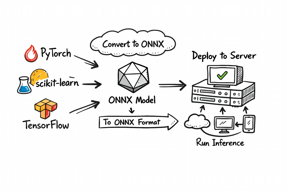
While mastering machine learning model training is paramount, the journey often falters during deployment across varied environments. This is precisely where ONNX (Open Neural Network Exchange) emerges as a critical enabler. ONNX establishes a standardized, framework-agnostic format, empowering models trained in leading frameworks such as PyTorch, TensorFlow, or scikit-learn for a single export and universal execution. This tutorial provides a detailed, step-by-step walkthrough of the complete ONNX workflow. We commence by fine-tuning a model and meticulously saving this refined version in both its native PyTorch format and the universally compatible ONNX format. Following this, we conduct a rigorous comparison of their inference performance on CPU, scrutinizing accuracy and inference speed to illuminate the practical advantages of framework-native models versus ONNX-based deployments. Furthermore, we demonstrate the conversion process for models trained with scikit-learn and TensorFlow, enabling you to extend this powerful deployment strategy across your entire machine learning ecosystem.

Mastering PyTorch Model Export to ONNX

This section focuses on fine-tuning a ResNet-18 model for image classification using the CIFAR-10 dataset. Subsequently, we will save this fine-tuned model in its native PyTorch format and also export it to the ONNX format. We will then execute both versions on CPU, comparing their inference results through accuracy and macro F1 score, alongside a thorough analysis of inference speed.

Essential Setup

Begin by installing the critical libraries required for model training, export, and benchmarking. We leverage PyTorch and TorchVision for model fine-tuning, ONNX for efficient model storage, and ONNX Runtime for high-performance ONNX inference on CPU. We also incorporate scikit-learn for its straightforward evaluation metrics, including accuracy and F1 score.

!pip install -q torch torchvision onnx onnxruntime scikit-learn
!pip install -q skl2onnx tensorflow tf2onnx protobuf

Next, import all essential modules to facilitate model training, export, and precise performance measurement.

import time
import numpy as np

import torch
import torch.nn as nn
from torch.utils.data import DataLoader
from torchvision import datasets, transforms, models

import onnx
import onnxruntime as ort

from sklearn.metrics import accuracy_score, f1_score

Loading CIFAR-10 and Constructing ResNet-18

Now, we prepare the dataset and model for training. The get_cifar10_loaders function efficiently loads CIFAR-10, returning optimized DataLoaders for both training and testing phases. To align with ResNet-18's architecture, which is designed for ImageNet-sized inputs, we resize CIFAR-10 images from their native 32×32 resolution to 224×224. We also apply ImageNet normalization values to ensure optimal utilization of the pretrained ResNet weights. To enhance model robustness, the training loader incorporates random horizontal flipping as a basic data augmentation technique.

def get_cifar10_loaders(batch_size: int = 64):
    """
    Returns train and test DataLoaders for CIFAR-10.
    We resize to 224x224 and use ImageNet normalization so ResNet18 works nicely.
    """
    imagenet_mean = [0.485, 0.456, 0.406]
    imagenet_std = [0.229, 0.224, 0.225]

    train_transform = transforms.Compose(
        [
            transforms.Resize((224, 224)),
            transforms.RandomHorizontalFlip(),
            transforms.ToTensor(),
            transforms.Normalize(mean=imagenet_mean, std=imagenet_std),
        ]
    )

    test_transform = transforms.Compose(
        [
            transforms.Resize((224, 224)),
            transforms.ToTensor(),
            transforms.Normalize(mean=imagenet_mean, std=imagenet_std),
        ]
    )

    train_dataset = datasets.CIFAR10(
        root="./data", train=True, download=True, transform=train_transform
    )
    test_dataset = datasets.CIFAR10(
        root="./data", train=False, download=True, transform=test_transform
    )

    train_loader = DataLoader(train_dataset, batch_size=batch_size, shuffle=True, num_workers=2)
    test_loader = DataLoader(test_dataset, batch_size=batch_size, shuffle=False, num_workers=2)

    return train_loader, test_loader

The build_resnet18_cifar10 function efficiently loads a ResNet-18 model pre-trained on ImageNet and precisely adapts the final fully connected layer. Whereas ImageNet comprises 1000 distinct classes, CIFAR-10 has only 10. Therefore, we reconfigure the last layer to output 10 logits, aligning it with the target dataset.

def build_resnet18_cifar10(num_classes: int = 10) -> nn.Module:
    """
    ResNet18 backbone with ImageNet weights, but final layer adapted to CIFAR-10.
    """
    weights = models.ResNet18_Weights.IMAGENET1K_V1
    model = models.resnet18(weights=weights)

    in_features = model.fc.in_features
    model.fc = nn.Linear(in_features, num_classes)
    return model

Accelerated Fine-Tuning for Benchmarking

This critical step involves a brief fine-tuning session to enable the model to adapt effectively to the CIFAR-10 dataset. This is not intended as a comprehensive training pipeline but rather a rapid demonstration loop, facilitating subsequent comparisons between PyTorch and ONNX inference. The quick_finetune_cifar10 function trains the model for a limited number of batches. It employs cross-entropy loss, suitable for multi-class classification tasks like CIFAR-10, and utilizes the Adam optimizer for rapid learning. The training loop iterates through batches, executes a forward pass, computes the loss, performs backpropagation, and updates model weights. Upon completion, it presents the average training loss, confirming that the training process has yielded tangible results.

def quick_finetune_cifar10(
    model: nn.Module,
    train_loader: DataLoader,
    device: torch.device,
    max_batches: int = 200,
):
    """
    Very light fine-tuning on CIFAR-10 to make metrics non-trivial.
    Trains for max_batches only (1 pass over subset of train data).
    """
    model.to(device)
    model.train()

    criterion = nn.CrossEntropyLoss()
    optimizer = torch.optim.Adam(model.parameters(), lr=1e-3)

    running_loss = 0.0
    for batch_idx, (images, labels) in enumerate(train_loader):
        if batch_idx >= max_batches:
            break

        images = images.to(device)
        labels = labels.to(device)

        optimizer.zero_grad()
        outputs = model(images)
        loss = criterion(outputs, labels)
        loss.backward()
        optimizer.step()

        running_loss += loss.item()

    avg_loss = running_loss / max_batches
    print(f"[Train] Average loss over {max_batches} batches: {avg_loss:.4f}")



device = torch.device("cuda" if torch.cuda.is_available() else "cpu")
print("Using device for training:", device)

train_loader, test_loader = get_cifar10_loaders(batch_size=64)

model = build_resnet18_cifar10(num_classes=10)
print("Starting quick fine-tuning on CIFAR-10 (demo)...")
quick_finetune_cifar10(model, train_loader, device, max_batches=200)

# Save weights for reuse (PyTorch + ONNX export)
torch.save(model.state_dict(), "resnet18_cifar10.pth")
print("✅ Saved fine-tuned weights to resnet18_cifar10.pth")

Following the training process, we efficiently save the model weights using torch.save(), generating a .pth file—the standard format for PyTorch model parameters.

Using device for training: cuda
Starting quick fine-tuning on CIFAR-10 (demo)...
[Train] Average loss over 200 batches: 0.7803
✅ Saved fine-tuned weights to resnet18_cifar10.pth

Efficient Export to ONNX Format

Now, we proceed with exporting the fine-tuned PyTorch model into the ONNX format, enabling its deployment and execution via ONNX Runtime. The export_resnet18_cifar10_to_onnx function efficiently loads the model architecture, integrates the fine-tuned weights, and crucially switches the model to evaluation mode using model.eval() to ensure consistent inference behavior. Furthermore, we construct a dummy input tensor with dimensions (1, 3, 224, 224). This dummy input is essential for the ONNX export process, as it allows the tool to trace the model graph and precisely ascertain input and output shapes.

def export_resnet18_cifar10_to_onnx(
    weights_path: str = "resnet18_cifar10.pth",
    onnx_path: str = "resnet18_cifar10.onnx",
):
    device = torch.device("cpu")  # export on CPU

    model = build_resnet18_cifar10(num_classes=10).to(device)
    model.load_state_dict(torch.load(weights_path, map_location=device))
    model.eval()

    # Dummy input (batch_size=1)
    dummy_input = torch.randn(1, 3, 224, 224, device=device)

    input_names = ["input"]
    output_names = ["logits"]
    dynamic_axes = {
        "input": {0: "batch_size"},
        "logits": {0: "batch_size"},
    }

    torch.onnx.export(
        model,
        dummy_input,
        onnx_path,
        export_params=True,
        opset_version=17,
        do_constant_folding=True,
        input_names=input_names,
        output_names=output_names,
        dynamic_axes=dynamic_axes,
    )

    print(f"✅ Exported ResNet18 (CIFAR-10) to ONNX: {onnx_path}")


export_resnet18_cifar10_to_onnx()

Finally, the torch.onnx.export() function generates the .onnx file, completing the export process.

✅ Exported ResNet18 (CIFAR-10) to ONNX: resnet18_cifar10.onnx

Benchmarking PyTorch CPU vs. ONNX Runtime Performance

In this concluding phase, we rigorously evaluate both formats side-by-side, ensuring all operations remain on CPU for a fair and conclusive comparison. The following function systematically executes four critical tasks: 1) loading the PyTorch model onto the CPU; 2) loading and validating the ONNX model; 3) verifying output similarity on a representative batch; and 4) performing warmup runs followed by precise inference speed benchmarking. We then execute timed inference over a predetermined number of batches: measuring the inference time for PyTorch on CPU and the corresponding time for ONNX Runtime on CPU. Concurrently, we collect predictions from both formats to compute accuracy and macro F1 scores. Finally, we present a detailed summary of average latency per batch and an estimated speedup ratio, highlighting the performance gains achieved with ONNX.

def verify_and_benchmark(
    weights_path: str = "resnet18_cifar10.pth",
    onnx_path: str = "resnet18_cifar10.onnx",
    batch_size: int = 64,
    warmup_batches: int = 2,
    max_batches: int = 30,
):
    device = torch.device("cpu")  # fair CPU vs CPU comparison
    print("Using device for evaluation:", device)

    # 1) Load PyTorch model
    torch_model = build_resnet18_cifar10(num_classes=10).to(device)
    torch_model.load_state_dict(torch.load(weights_path, map_location=device))
    torch_model.eval()

    # 2) Load ONNX model and create session
    onnx_model = onnx.load(onnx_path)
    onnx.checker.check_model(onnx_model)
    print("✅ ONNX model is well-formed.")

    ort_session = ort.InferenceSession(onnx_path, providers=["CPUExecutionProvider"])
    print("ONNXRuntime providers:", ort_session.get_providers())

    # 3) Data loader (test set)
    _, test_loader = get_cifar10_loaders(batch_size=batch_size)

    # -------------------------
    # A) Numeric closeness check on a single batch
    # -------------------------
    images, labels = next(iter(test_loader))
    images = images.to(device)
    labels = labels.to(device)

    with torch.no_grad():
        torch_logits = torch_model(images).cpu().numpy()

    ort_inputs = {"input": images.cpu().numpy().astype(np.float32)}
    ort_logits = ort_session.run(["logits"], ort_inputs)[0]

    abs_diff = np.abs(torch_logits - ort_logits)
    max_abs = abs_diff.max()
    mean_abs = abs_diff.mean()
    print(f"Max abs diff:  {max_abs:.6e}")
    print(f"Mean abs diff: {mean_abs:.6e}")

    # Relaxed tolerance to account for small numerical noise
    np.testing.assert_allclose(torch_logits, ort_logits, rtol=1e-02, atol=1e-04)
    print("✅ Outputs match closely between PyTorch and ONNXRuntime within relaxed tolerance.")

    # -------------------------
    # B) Warmup runs (on a couple of batches, not recorded)
    # -------------------------
    print(f"\
Warming up on {warmup_batches} batches (not timed)...")
    warmup_iter = iter(test_loader)
    for _ in range(warmup_batches):
        try:
            imgs_w, _ = next(warmup_iter)
        except StopIteration:
            break
        imgs_w = imgs_w.to(device)

        with torch.no_grad():
            _ = torch_model(imgs_w)

        _ = ort_session.run(["logits"], {"input": imgs_w.cpu().numpy().astype(np.float32)})

    # -------------------------
    # C) Timed runs + metric collection
    # -------------------------
    print(f"\
Running timed evaluation on up to {max_batches} batches...")
    all_labels = []
    torch_all_preds = []
    onnx_all_preds = []

    torch_times = []
    onnx_times = []

    n_batches = 0
    for batch_idx, (images, labels) in enumerate(test_loader):
        if batch_idx >= max_batches:
            break

        n_batches += 1
        images = images.to(device)
        labels = labels.to(device)

        # Time PyTorch
        start = time.perf_counter()
        with torch.no_grad():
            torch_out = torch_model(images)
        end = time.perf_counter()
        torch_times.append(end - start)

        # Time ONNX
        ort_inp = {"input": images.cpu().numpy().astype(np.float32)}
        start = time.perf_counter()
        ort_out = ort_session.run(["logits"], ort_inp)[0]
        end = time.perf_counter()
        onnx_times.append(end - start)

        # Predictions
        torch_pred_batch = torch_out.argmax(dim=1).cpu().numpy()
        onnx_pred_batch = ort_out.argmax(axis=1)

        labels_np = labels.cpu().numpy()

        all_labels.append(labels_np)
        torch_all_preds.append(torch_pred_batch)
        onnx_all_preds.append(onnx_pred_batch)

    if n_batches == 0:
        print("No batches processed for evaluation. Check max_batches / dataloader.")
        return

    # Concatenate across batches
    all_labels = np.concatenate(all_labels, axis=0)
    torch_all_preds = np.concatenate(torch_all_preds, axis=0)
    onnx_all_preds = np.concatenate(onnx_all_preds, axis=0)

    # -------------------------
    # D) Metrics: accuracy & F1 (macro)
    # -------------------------
    torch_acc = accuracy_score(all_labels, torch_all_preds) * 100.0
    onnx_acc = accuracy_score(all_labels, onnx_all_preds) * 100.0

    torch_f1 = f1_score(all_labels, torch_all_preds, average="macro") * 100.0
    onnx_f1 = f1_score(all_labels, onnx_all_preds, average="macro") * 100.0

    print("\
📊 Evaluation metrics on timed subset")
    print(f"PyTorch  - accuracy: {torch_acc:.2f}%   F1 (macro): {torch_f1:.2f}%")
    print(f"ONNX     - accuracy: {onnx_acc:.2f}%   F1 (macro): {onnx_f1:.2f}%")

    # -------------------------
    # E) Latency summary
    # -------------------------
    avg_torch = sum(torch_times) / len(torch_times)
    avg_onnx = sum(onnx_times) / len(onnx_times)

    print(f"\
⏱  Latency over {len(torch_times)} batches (batch size = {batch_size})")
    print(f"PyTorch avg:      {avg_torch * 1000:.2f} ms / batch")
    print(f"ONNXRuntime avg:  {avg_onnx * 1000:.2f} ms / batch")
    if avg_onnx > 0:
        print(f"Estimated speedup (Torch / ORT): {avg_torch / avg_onnx:.2f}x")
    else:
        print("Estimated speedup: N/A (onnx time is 0?)")

verify_and_benchmark(
    weights_path="resnet18_cifar10.pth",
    onnx_path="resnet18_cifar10.onnx",
    batch_size=64,
    warmup_batches=2,
    max_batches=30,
)

The outcome is a comprehensive report demonstrating identical accuracy metrics while showcasing significant improvements in inference speed with ONNX.

Using device for evaluation: cpu
✅ ONNX model is well-formed.
ONNXRuntime providers: ['CPUExecutionProvider']
Max abs diff:  3.814697e-06
Mean abs diff: 4.552072e-07
✅ Outputs match closely between PyTorch and ONNXRuntime within relaxed tolerance.

Warming up on 2 batches (not timed)...

Running timed evaluation on up to 30 batches...

📊 Evaluation metrics on timed subset
PyTorch  - accuracy: 78.18%   F1 (macro): 77.81%
ONNX     - accuracy: 78.18%   F1 (macro): 77.81%

⏱  Latency over 30 batches (batch size = 64)
PyTorch avg:      2192.50 ms / batch
ONNXRuntime avg:  1317.09 ms / batch
Estimated speedup (Torch / ORT): 1.66x

Broaden Your Reach: Exporting Scikit-Learn and Keras Models to ONNX

This section extends the utility of ONNX beyond deep learning frameworks, demonstrating its application to traditional machine learning models. We will export a standard scikit-learn Random Forest classifier and a TensorFlow/Keras neural network into ONNX format. This clearly illustrates ONNX's pivotal role as a unified deployment layer, bridging classical machine learning and advanced deep learning paradigms.

Seamless Export of Scikit-Learn Models to ONNX

We will now train a straightforward Random Forest classifier using scikit-learn on the Iris dataset, followed by its conversion to ONNX format for streamlined deployment. Prior to the conversion process, we meticulously define the ONNX input type, specifying the input name, floating-point data type, a dynamic batch size, and the precise number of input features. These specifications are imperative for ONNX to construct a static computation graph. Subsequently, we convert the trained model, save the resultant .onnx file, and finally, validate it to confirm that the exported model is structurally sound and fully prepared for inference with ONNX Runtime.

from sklearn.datasets import load_iris
from sklearn.model_selection import train_test_split
from sklearn.ensemble import RandomForestClassifier

from skl2onnx import convert_sklearn
from skl2onnx.common.data_types import FloatTensorType
import onnx

# 1) Train a small sklearn model
iris = load_iris()
X_train, X_test, y_train, y_test = train_test_split(
    iris.data, iris.target, test_size=0.2, random_state=42
)

rf = RandomForestClassifier(n_estimators=50, random_state=42)
rf.fit(X_train, y_train)
print("✅ Trained RandomForestClassifier on Iris")

# 2) Define input type for ONNX (batch_size x n_features)
n_features = X_train.shape[1]
initial_type = [("input", FloatTensorType([None, n_features]))]

# 3) Convert to ONNX
rf_onnx = convert_sklearn(rf, initial_types=initial_type, target_opset=17)

onnx_path_sklearn = "random_forest_iris.onnx"
with open(onnx_path_sklearn, "wb") as f:
    f.write(rf_onnx.SerializeToString())

# 4) Quick sanity check
onnx.checker.check_model(onnx.load(onnx_path_sklearn))
print(f"✅ Exported sklearn model to {onnx_path_sklearn}")

Our scikit-learn model is now fully trained, converted, securely saved, and rigorously validated.

✅ Trained RandomForestClassifier on Iris
✅ Exported sklearn model to random_forest_iris.onnx

Efficient Export of TensorFlow/Keras Models to ONNX

This section details the process of exporting a TensorFlow neural network to ONNX format, underscoring how deep learning models trained with TensorFlow can be efficiently prepared for universal deployment. The environment is meticulously configured for CPU execution with minimal logging to ensure a clean and reproducible process. A concise, fully connected Keras model is constructed using the Functional API, featuring a fixed input size and a limited number of layers to facilitate a straightforward conversion. An input signature is subsequently defined, providing ONNX with the necessary information regarding the expected input shape, data type, and tensor name for inference. Leveraging this data, the Keras model is converted into the ONNX format and saved as a .onnx file. Finally, the exported model undergoes validation to guarantee its structural integrity and readiness for execution via ONNX Runtime or any other compatible ONNX inference engine.

import os

os.environ["TF_CPP_MIN_LOG_LEVEL"] = "2" 
os.environ["CUDA_VISIBLE_DEVICES"] = "-1"

import tensorflow as tf
import tf2onnx
import onnx

# 3) Build a simple Keras model
inputs = tf.keras.Input(shape=(32,), name="input")
x = tf.keras.layers.Dense(64, activation="relu")(inputs)
x = tf.keras.layers.Dense(32, activation="relu")(x)
outputs = tf.keras.layers.Dense(10, activation="softmax", name="output")(x)
keras_model = tf.keras.Model(inputs=inputs, outputs=outputs)
keras_model.summary()

# 4) Convert to ONNX
spec = (
    tf.TensorSpec(
        keras_model.inputs[0].shape,
        keras_model.inputs[0].dtype,
        name="input",
    ),
)

onnx_model_keras, _ = tf2onnx.convert.from_keras(
    keras_model,
    input_signature=spec,
    opset=17,
)

onnx_path_keras = "keras_mlp.onnx"
with open(onnx_path_keras, "wb") as f:
    f.write(onnx_model_keras.SerializeToString())

onnx.checker.check_model(onnx.load(onnx_path_keras))
print(f"✅ Exported Keras/TensorFlow model to {onnx_path_keras}")

Our TensorFlow/Keras model is now fully trained, converted, securely saved, and rigorously validated.

Model: "functional_4"

┏━━━━━━━━━━━━━━━━━━━━━━━━━━━━━━━━━┳━━━━━━━━━━━━━━━━━━━━━━━━┳━━━━━━━━━━━━━━━┓
┃ Layer (type)                    ┃ Output Shape           ┃       Param # ┃
┡━━━━━━━━━━━━━━━━━━━━━━━━━━━━━━━━━╇━━━━━━━━━━━━━━━━━━━━━━━━╇━━━━━━━━━━━━━━━┩
│ input (InputLayer)              │ (None, 32)             │             0 │
├─────────────────────────────────┼────────────────────────┼───────────────┤
│ dense_8 (Dense)                 │ (None, 64)             │         2,112 │
├─────────────────────────────────┼────────────────────────┼───────────────┤
│ dense_9 (Dense)                 │ (None, 32)             │         2,080 │
├─────────────────────────────────┼────────────────────────┼───────────────┤
│ output (Dense)                  │ (None, 10)             │           330 │
└─────────────────────────────────┴────────────────────────┴───────────────┘

Total params: 4,522 (17.66 KB)

Trainable params: 4,522 (17.66 KB)

Non-trainable params: 0 (0.00 B)

✅ Exported Keras/TensorFlow model to keras_mlp.onnx

Conclusion: Embrace ONNX for Unified ML Deployment

ONNX serves as an indispensable bridge, seamlessly connecting the model training phase with robust real-world deployment by ensuring model portability, framework independence, and optimized inference capabilities. Through the process of fine-tuning a PyTorch model, exporting it to ONNX, and conducting a comparative analysis of accuracy and CPU inference speed, we have empirically demonstrated that ONNX consistently delivers equivalent predictive quality while significantly enhancing performance. This standardization simplifies the pathway from initial experimentation to production-ready deployment, effectively minimizing friction and streamlining the integration of models across diverse operational environments. Given this unparalleled level of portability, performance, and consistency, adopting ONNX for all your machine learning projects is no longer just an option, but a strategic imperative.