


This definitive guide empowers you to cluster text documents with unparalleled accuracy using state-of-the-art large language model embeddings and robust scikit-learn clustering algorithms. Explore essential topics including: Why LLM-based embeddings excel in document clustering. How to generate precise embeddings from raw text via pre-trained sentence transformers. Effective application and comparison of K-Means and DBSCAN for clustering embedded documents. Let's dive directly into the core strategies.
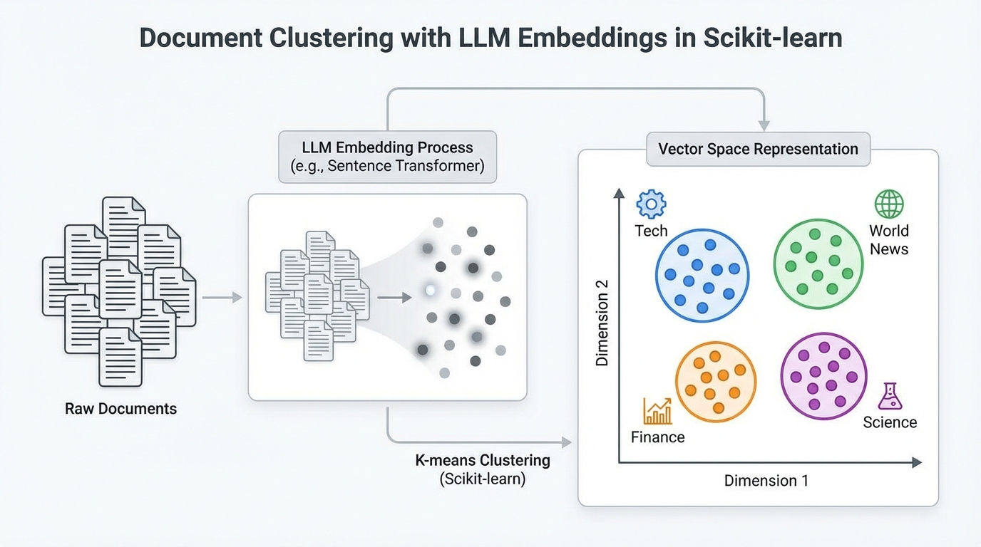
Master Document Clustering with LLM Embeddings in Scikit-learn (Click to enlarge)
Image by Editor
Unlocking Textual Insights: The Power of LLM Embeddings for Clustering
Encountering a vast corpus of unclassified documents and tasked with precise topical grouping? Traditional text clustering methods, while functional, often falter due to inherent limitations. These include TF-IDF's reliance on word frequency, neglecting semantic depth, and Word2Vec's focus on individual word relationships, overlooking nuanced full-text context. In stark contrast, advanced embeddings from large language models, particularly sentence transformers, offer superior semantic capture. They distinguish subtle meanings (e.g., natural vs. decision trees) and encode holistic, document-level understanding. Crucially, these embeddings leverage extensive pre-training on massive text datasets, embedding significant linguistic knowledge.
Building upon our prior tutorial on leveraging LLM embeddings as potent features for scikit-learn models, this exploration concentrates specifically on employing document embeddings for sophisticated similarity-based clustering. Our objective is to precisely identify common themes within related documents.
Comprehensive Workflow: A Step-by-Step Python Implementation
Embark on the complete clustering process with this detailed Python walkthrough. Depending on your specific environment, you might need to install prerequisite libraries using pip install. Assuming successful setup, we commence by importing essential modules and classes, notably KMeans, scikit-learn's premier implementation for the k-means clustering algorithm.
| 12345678910111213 | import pandas as pdimport numpy as npfrom sentence_transformers import SentenceTransformerfrom sklearn.cluster import KMeansfrom sklearn.decomposition import PCAfrom sklearn.metrics import silhouette_score, adjusted_rand_scorefrom sklearn.preprocessing import LabelEncoderimport matplotlib.pyplot as pltimport seaborn as sns # Configurations for clearer visualizationssns.set_style("whitegrid")plt.rcParams['figure.figsize'] = (12, 6) |
Effortless Dataset Loading and Initial Analysis
Next, we strategically load the dataset. We utilize a comprehensive BBC News dataset, pre-labeled by topic and readily accessible from a public Google-hosted repository. This step allows us to inspect the ground-truth topic assignments and ascertain the dataset's scale, currently comprising 2,225 documents. The dataset's categories provide a foundational understanding of the inherent topical structure.
| 123456 | url = "https://storage.googleapis.com/dataset-uploader/bbc/bbc-text.csv"df = pd.read_csv(url) print(f"Dataset loaded: {len(df)} documents")print(f"Categories: {df['category'].unique()} ")print(df['category'].value_counts()) |
With the data loaded, we are optimally positioned for the two pivotal stages of our workflow: generating sophisticated embeddings from raw text and subsequently clustering these powerful embeddings.
Seamless Embedding Generation with a Pre-Trained Model
Leveraging specialized libraries like sentence_transformers simplifies the process of utilizing pre-trained models for generating embeddings. Our approach involves loading an appropriate model, such as the efficient all-MiniLM-L6-v2, which is expertly trained to produce 384-dimensional embeddings. We then execute inference across the entire dataset, transforming each document into a precise numerical vector that profoundly captures its semantic essence.
We initiate this by loading the model:
| 123456 | # Load embeddings model (downloaded automatically on first use)print("Loading embeddings model...")model = SentenceTransformer('all-MiniLM-L6-v2') # This model converts text into a 384-dimensional vectorprint(f"Model loaded. Embedding dimension: {model.get_sentence_embedding_dimension()}") |
Subsequently, we efficiently generate embeddings for the entirety of our document collection:
| 123456789101112 | # Convert all documents into embedding vectorsprint("Generating embeddings (this may take a few minutes)...") texts = df['text'].tolist()embeddings = model.encode( texts, show_progress_bar=True, batch_size=32 # Batch processing for efficiency) print(f"Embeddings generated: matrix size is {embeddings.shape}")print(f" → Each document is now represented by {embeddings.shape[1]} numeric values") |
Crucially, remember that an embedding is a high-dimensional numerical vector. Documents exhibiting semantic similarity will naturally possess embeddings that reside in close proximity within this sophisticated vector space.
Advanced Clustering of Document Embeddings with K-Means
Applying scikit-learn's sophisticated k-means clustering algorithm is remarkably straightforward. We simply input the embedding matrix and precisely specify the desired number of clusters. While k-means requires this number as a prerequisite, we can leverage our dataset's known ground-truth categories in this specific example. For other scenarios, advanced techniques like the elbow method are invaluable for guiding this critical selection.
The subsequent code expertly applies k-means and rigorously evaluates the outcomes using multiple metrics, prominently featuring the Adjusted Rand Index (ARI). ARI serves as a permutation-invariant measure that meticulously compares the generated cluster assignments against the authoritative true category labels. Consequently, scores closer to 1 signify a superior alignment with the ground truth.
| 12345678910111213 | n_clusters = 5 kmeans = KMeans(n_clusters=n_clusters, random_state=42, n_init=10)kmeans_labels = kmeans.fit_predict(embeddings) # Evaluation against ground-truth categoriesle = LabelEncoder()true_labels = le.fit_transform(df['category']) print(" K-Means Results:")print(f" Silhouette Score: {silhouette_score(embeddings, kmeans_labels):.3f}")print(f" Adjusted Rand Index: {adjusted_rand_score(true_labels, kmeans_labels):.3f}")print(f" Distribution: {pd.Series(kmeans_labels).value_counts().sort_index().tolist()}") |
Example output:
| 1234 | K-Means Results: Silhouette Score: 0.066 Adjusted Rand Index: 0.899 Distribution: [376, 414, 517, 497, 421] |
Exploring Document Clustering with DBSCAN
Alternatively, we can deploy DBSCAN, a sophisticated density-based clustering algorithm that intelligently infers the optimal number of clusters based on point density. Rather than requiring a pre-specified cluster count, DBSCAN necessitates critical parameter tuning, including eps (the neighborhood radius) and min_samples.
| 12345678910111213141516 | from sklearn.cluster import DBSCAN # DBSCAN often works better with cosine distance for text embeddingsdbscan = DBSCAN(eps=0.5, min_samples=5, metric='cosine')dbscan_labels = dbscan.fit_predict(embeddings) # Count clusters (-1 indicates noise points)n_clusters_found = len(set(dbscan_labels)) - (1 if -1 in dbscan_labels else 0)n_noise = list(dbscan_labels).count(-1) print("\nDBSCAN Results:")print(f" Clusters found: {n_clusters_found}")print(f" Noise documents: {n_noise}")print(f" Silhouette Score: {silhouette_score(embeddings[dbscan_labels != -1], dbscan_labels[dbscan_labels != -1]):.3f}")print(f" Adjusted Rand Index: {adjusted_rand_score(true_labels, dbscan_labels):.3f}")print(f" Distribution: {pd.Series(dbscan_labels).value_counts().sort_index().to_dict()}") |
DBSCAN's performance is notably sensitive to its hyperparameters; achieving optimal results frequently necessitates systematic tuning via robust search strategies. Once effective parameters are identified, a visual comparison of the clustering outputs becomes highly informative. The ensuing code strategically projects the embeddings into a two-dimensional space using principal component analysis (PCA), followed by plotting the true categories alongside the K-Means and DBSCAN cluster assignments.
| 1234567891011121314151617181920212223242526272829303132333435363738394041424344454647484950515253 | # Reduce embeddings to 2D for visualizationpca = PCA(n_components=2, random_state=42)embeddings_2d = pca.fit_transform(embeddings) # Create comparative visualizationfig, axes = plt.subplots(1, 3, figsize=(18, 5)) # Plot 1: True categoriescategory_colors = {cat: i for i, cat in enumerate(df['category'].unique())}color_map = df['category'].map(category_colors) axes[0].scatter( embeddings_2d[:, 0], embeddings_2d[:, 1], c=color_map, cmap='Set2', alpha=0.6, s=30)axes[0].set_title('True Categories', fontsize=12, fontweight='bold')axes[0].set_xlabel('PC1')axes[0].set_ylabel('PC2') # Plot 2: K-Meansscatter2 = axes[1].scatter( embeddings_2d[:, 0], embeddings_2d[:, 1], c=kmeans_labels, cmap='viridis', alpha=0.6, s=30)axes[1].set_title(f'K-Means (k={n_clusters})', fontsize=12, fontweight='bold')axes[1].set_xlabel('PC1')axes[1].set_ylabel('PC2')plt.colorbar(scatter2, ax=axes[1]) # Plot 3: DBSCANscatter3 = axes[2].scatter( embeddings_2d[:, 0], embeddings_2d[:, 1], c=dbscan_labels, cmap='plasma', alpha=0.6, s=30)axes[2].set_title(f'DBSCAN ({n_clusters_found} clusters + noise)', fontsize=12, fontweight='bold')axes[2].set_xlabel('PC1')axes[2].set_ylabel('PC2')plt.colorbar(scatter3, ax=axes[2]) plt.tight_layout()plt.show() |
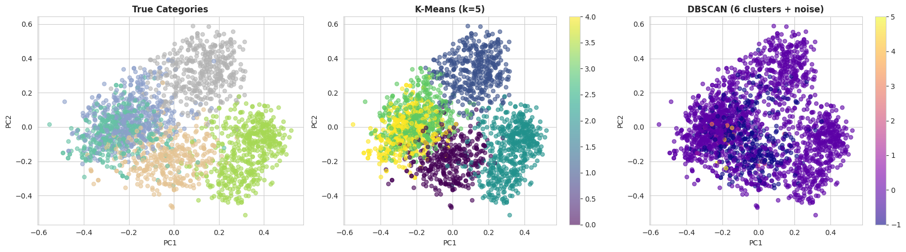
With the default DBSCAN parameters, k-means generally demonstrates superior performance on this specific dataset. This disparity arises primarily from two factors: DBSCAN's susceptibility to the curse of dimensionality, making it challenging with 384-dimensional embeddings, and k-means' inherent effectiveness with relatively well-separated clusters, a characteristic clearly present in the BBC News dataset's distinct topical structure.
Concluding Your Clustering Journey
This comprehensive article has meticulously guided you through the process of effectively clustering a diverse collection of text documents. We have masterfully transformed raw text into sophisticated embedding representations generated by cutting-edge pre-trained large language models. Following this transformation, we successfully applied and evaluated traditional clustering techniques—k-means and DBSCAN—to group semantically coherent documents and rigorously assess their performance against established topic labels.